쉐비 콜로라도 배터리 자가 교체를 위한 시뮬레이션
by Justin Kim
현재 제가 운행 중인 쉐보레 콜로라도는 덩치도 크고 공간도 넓어서 다방면으로 정말 유용하게 잘 활용하고 있는 차량입니다. 특히 요즘에는 출퇴근용으로 매일같이 운행하고 있는데, 최근 들어 부쩍 배터리 방전이 잦아졌습니다. 아침마다 출근하려는데 시동이 걸리지 않아 직접 점프 스타트 장비를 연결해 시동을 거는 일이 반복되다 보니, 여간 번거로운 것이 아니었습니다.
이제 4년 차에 접어든 차량이라 배터리 수명 자체가 완전히 다했다고 보기에는 기간이 조금 짧은 듯한 느낌이 들었습니다. 보통 배터리 교체 주기를 생각하면 조금 더 사용할 수 있어야 하는데, 자꾸 방전이 반복되는 것을 보며 결국 제 운행 패턴에 문제가 있는 것이 아닐까 하는 의구심이 생겼지만 운행 패턴을 하루아침에 바꾸는 것은 현실적으로 불가능한 일이었습니다. 결국 환경을 바꿀 수 없다면, 저의 가혹한(?) 운행 환경을 충분히 감당해낼 수 있는 적합한 배터리로 교체하는 것이 해결책이라는 결론을 내리게 되었습니다.
가설 수립 및 검증
교체할 배터리를 선택하기에 앞서, 제 운행 환경을 분석하고 가설을 세워보았습니다.
- 운행 패턴: 하루 2회 운행. 90%는 10분 이내의 단거리 주행, 10% 정도만 비정기적인 1시간 이상 주행.
- 문제 현상: 일주일에 한 번 정도 방전 발생 (70Ah 순정 배터리 기준).
- 가설: 시동 시 소모된 전력을 10분 미만의 짧은 주행으로는 알터네이터가 충분히 보충하지 못한다. 여기에 블랙박스 주차 모드 등의 암전류가 더해져 배터리 잔량(SoC)이 계단식으로 하락할 것이다. 용량을 키우면 이 하락 기울기를 버티는 버퍼가 커져 방전 주기를 늦출 수 있을 것이다.
이 가설을 검증하기 위해 파이썬으로 초 단위(Second-by-second) 시뮬레이션을 수행해보았습니다. 특히 배터리 잔량이 시동 한계(약 20Ah) 이하로 떨어지면 ‘점프 스타트’를 통해 외부 전원으로 시동을 걸고 충전을 시작한다는 현실적인 시나리오를 적용했습니다.
import matplotlib.pyplot as plt
import numpy as np
import random

def simulate_battery_second_by_second(capacity_ah, days=30, charge_efficiency=1.0):
    # Time step: 1 second
    total_seconds = days * 24 * 3600

    # Parameters
    current_charge_ah = capacity_ah

    # Threshold for Cranking (Below this, we need a jump start)
    # Fixed 20Ah needed to crank safely
    min_start_threshold_ah = 20.0

    # Current Draw / Charge rates (Amps)
    parasitic_drain_amp = 0.35  # Parking mode
    alternator_charge_amp = 20.0 # Effective charge during drive

    # Start consumption (Ah per start)
    start_cost_ah = 0.2

    # Trip Config
    # Define approximate start times for trips (e.g., 8am and 6pm) in seconds from midnight
    trip_start_times_sec = [8 * 3600, 18 * 3600]

    # Pre-calculate trip schedule for the entire period to save processing time
    # We will store events as a list of (start_second, duration_seconds)
    trip_events = []

    for day in range(days):
        day_offset = day * 24 * 3600
        for start_time_local in trip_start_times_sec:
            # Add some randomness to start time (+/- 30 mins)
            actual_start = day_offset + start_time_local + random.randint(-1800, 1800)

            # Determine duration
            # 90% short trips (5-10 mins)
            # 10% long trips (Normal dist: mean=60m, std=10m)
            if random.random() < 0.9:
                # Uniform 5~10 mins
                duration_min = random.uniform(5, 10)
            else:
                # Normal distribution 60 mins
                duration_min = np.random.normal(60, 10)
                if duration_min < 5: duration_min = 5 # Clamp min

            duration_sec = int(duration_min * 60)
            trip_events.append((actual_start, duration_sec))

    # Sort events just in case
    trip_events.sort()

    history_hours = []
    history_soc = []
    jump_start_events = [] # To track when jump starts happened

    # To speed up, we can calculate state between events instead of looping every second
    # State 0: Parking
    # State 1: Driving

    evt_idx = 0
    num_events = len(trip_events)
    current_time = 0

    # Record history every hour (3600 ticks) for plotting resolution
    record_interval = 3600
    next_record_time = 0

    while current_time < total_seconds:
        # Determine next event start
        if evt_idx < num_events:
            next_evt_start, next_evt_duration = trip_events[evt_idx]
        else:
            next_evt_start = total_seconds + 1 # End of sim

        # 1. PARKING Phase (current_time -> next_evt_start)
        parking_duration = next_evt_start - current_time

        # Calculate drain for this parking block
        # Check if we cross recording intervals

        # Simplified loop for recording resolution
        while current_time < next_evt_start and current_time < total_seconds:
            step = min(record_interval, next_evt_start - current_time)

            # Apply Drain
            # Ah = Amps * Hours
            drain_ah = parasitic_drain_amp * (step / 3600.0)
            current_charge_ah -= drain_ah

            # Clamp min to start threshold (User logic: cannot go below failure point)
            if current_charge_ah < min_start_threshold_ah:
                current_charge_ah = min_start_threshold_ah

            current_time += step

            # Record if we hit a boundary (approx)
            if current_time >= next_record_time:
                history_hours.append(current_time / 3600.0)
                history_soc.append(current_charge_ah)
                next_record_time += record_interval

        if evt_idx >= num_events:
            break

        # 2. DRIVING Phase (Start + Charge)

        # Check if we have enough juice to start
        if current_charge_ah <= min_start_threshold_ah:
             # JUMP START SCENARIO
             # External power used. No drain.
             # Ensure we start at least at the threshold
             current_charge_ah = min_start_threshold_ah
             jump_start_events.append(current_time / 3600.0)
        else:
            # NORMAL START SCENARIO
            current_charge_ah -= start_cost_ah
            # Check floor again just in case start cost dips it
            if current_charge_ah < min_start_threshold_ah:
                current_charge_ah = min_start_threshold_ah
                # If start cost dipped it, technically it failed to start without help?
                # But let's assume it cranked barely.

        # Charge during drive
        # We assume driving happens instantly for the sake of the 'while' loop step,
        # or we integrate it. Let's integrate it.

        drive_end_time = current_time + next_evt_duration

        while current_time < drive_end_time and current_time < total_seconds:
            step = min(record_interval, drive_end_time - current_time)

            # Apply Charge (Modified by Efficiency)
            charge_ah = (alternator_charge_amp * charge_efficiency) * (step / 3600.0)
            current_charge_ah += charge_ah

            # Clamp max
            if current_charge_ah > capacity_ah: current_charge_ah = capacity_ah

            current_time += step

            if current_time >= next_record_time:
                history_hours.append(current_time / 3600.0)
                history_soc.append(current_charge_ah)
                next_record_time += record_interval

        evt_idx += 1

    return history_hours, history_soc, jump_start_events

def run_capacity_simulation():
    days = 30
    capacities = [70, 80, 90]
    colors = {70: '#ff4d4d', 80: '#ffca28', 90: '#66bb6a'}

    plt.figure(figsize=(10, 6))

    seed_val = 42

    for cap in capacities:
        random.seed(seed_val)
        np.random.seed(seed_val)
        hours, soc, jumps = simulate_battery_second_by_second(cap, days, charge_efficiency=1.0)

        plt.plot(hours, soc, label=f'{cap}Ah Battery', color=colors[cap], linewidth=1.5)

        # Mark jump starts with an 'x'
        if jumps:
             plt.scatter(jumps, [soc[int(t)] for t in [min(int(j), len(soc)-1) for j in jumps] if int(t) < len(soc)],
                         color=colors[cap], marker='x', s=50, zorder=5) # Crude approx for Y pos

    # Plot risk threshold line (Fixed 20Ah)
    plt.axhline(y=20, color='gray', linestyle='--', alpha=0.5, label='Start Threshold (20Ah)')

    plt.title('Battery SoC Simulation: Capacity Difference (Efficiency 100%)')
    plt.xlabel('Hours Passed (30 Days)')
    plt.ylabel('State of Charge (Ah)')
    plt.grid(True, linestyle=':', alpha=0.6)
    plt.legend()
    plt.tight_layout()

    output_path = 'battery_simulation.png'
    plt.savefig(output_path, dpi=150)
    print(f"Capacity Simulation graph saved to {output_path}")

def run_efficiency_simulation():
    days = 30
    capacity = 95
    scenarios = [
        {'type': 'Standard Lead-Acid', 'eff': 0.7, 'color': '#ff4d4d'},
        {'type': 'AGM Battery', 'eff': 0.9, 'color': '#007bff'}
    ]

    plt.figure(figsize=(10, 6))

    seed_val = 42 # Same driving pattern

    for sc in scenarios:
        random.seed(seed_val)
        np.random.seed(seed_val)

        hours, soc, jumps = simulate_battery_second_by_second(capacity, days, charge_efficiency=sc['eff'])

        label_text = f"95Ah {sc['type']} (Eff: {int(sc['eff']*100)}%)"
        plt.plot(hours, soc, label=label_text, color=sc['color'], linewidth=2)

        if jumps:
             plt.scatter(jumps, [soc[int(t)] for t in [min(int(j), len(soc)-1) for j in jumps] if int(t) < len(soc)],
                         color=sc['color'], marker='x', s=50, zorder=5)

    plt.axhline(y=20, color='gray', linestyle='--', alpha=0.5, label='Start Threshold (20Ah)')

    plt.title('Battery SoC Simulation: Charging Efficiency (Standard vs AGM)')
    plt.xlabel('Hours Passed (30 Days)')
    plt.ylabel('State of Charge (Ah)')
    plt.grid(True, linestyle=':', alpha=0.6)
    plt.legend()
    plt.tight_layout()

    output_path = 'charging_efficiency_simulation.png'
    plt.savefig(output_path, dpi=150)
    print(f"Efficiency Simulation graph saved to {output_path}")

if __name__ == "__main__":
    # We display the run logic here, but in the blog we might hide the main block or show it.
    # The snippet in the blog shows up to the functions.
    run_capacity_simulation()
    run_efficiency_simulation()
시뮬레이션 결과(30일 추이)는 다음과 같습니다.
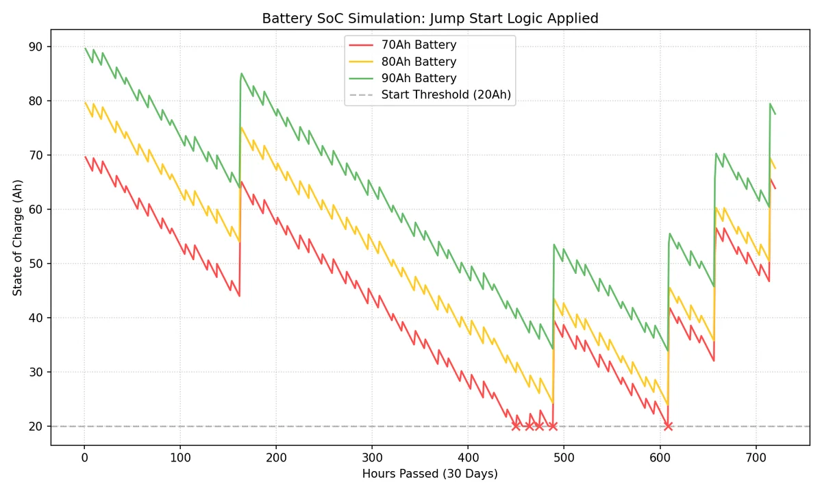
그래프를 보면 70Ah 배터리(적색)는 주차 중 암전류로 인해 잔량이 지속적으로 감소하다가, 시동 한계선(20Ah)에 도달하면 더 이상 내려가지 않고 멈춥니다(점프 스타트 개입). 이후 주행을 통해 잠시 회복하지만 곧 다시 바닥으로 떨어지는 위태로운 모습을 보입니다. 반면 90Ah 배터리(녹색)는 동일한 조건에서도 여유 있는 용량 덕분에 한계선 위에서 안정적으로 사이클을 유지합니다.
충전 효율의 점검
단순히 배터리 용량만 키운다고 해서 모든 문제가 해결될지 의문이 들었습니다. 충전이 소모를 따라가지 못하는 근본적인 환경이라면, 결국 큰 배터리도 방전 시점만 늦출 뿐이기 때문입니다. 그래서 한 가지 더 확인해보고 싶었던 것이 바로 충전 효율입니다. 짧은 주행 시간 동안 얼마나 효율적으로 에너지를 받아들일 수 있는지, 효율 변수를 조정하여 다시 한번 시뮬레이션을 진행해 보았습니다.
일반적인 납산 배터리의 충전 효율(Coulombic Efficiency)은 약 70%~85% 수준입니다. 즉, 시동 시 소모된 1Ah를 복구하기 위해 발전기는 약 1.2~1.4Ah 이상의 에너지를 밀어넣어야 합니다. 하지만 단거리 주행에서는 배터리 내부 저항으로 인해 전하를 받아들이는 속도가 제한되어, 실제 충전량은 시뮬레이션보다 더 낮을 가능성이 큽니다.
차량용 배터리 타입별 충전 성능을 비교하면 다음과 같습니다.
| 배터리 타입 | 예상 충전 효율 | 특징 |
|---|---|---|
| 일반 납산 (Flooded) | 약 70% ~ 85% | 표준적인 성능 |
| EFB (Enhanced Flooded) | 약 85% ~ 90% | 납산 배터리의 내구성을 보완 |
| AGM (Absorbent Glass Mat) | 약 90% 이상 | 충전 속도가 매우 빠르고 저온 시동성이 뛰어남 |
일단 국내 쇼핑몰을 검색하니, EFB는 거의 없고 AGM만이 대부분이었습니다. 그래서 AGM으로 교체하는 것이 현실적인 선택이 될것이라고 생각하고 다시 시뮬레이션을 진행해 보았습니다.
시뮬레이션 결과는 다음과 같습니다.
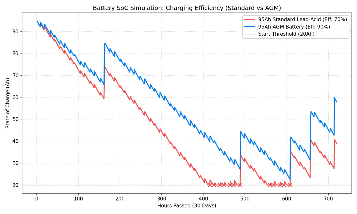
그래프를 보면 95Ah 납산 배터리(적색, 효율 70%)는 용량은 크지만 충전 속도가 따라가지 못해 결국 방전 위험선에 도달하는 반면, 95Ah AGM 배터리(청색, 효율 90%)는 빠른 충전 회복력 덕분에 훨씬 안정적인 잔량을 유지할 것을 기대할 수 있습니다.
교체 시작
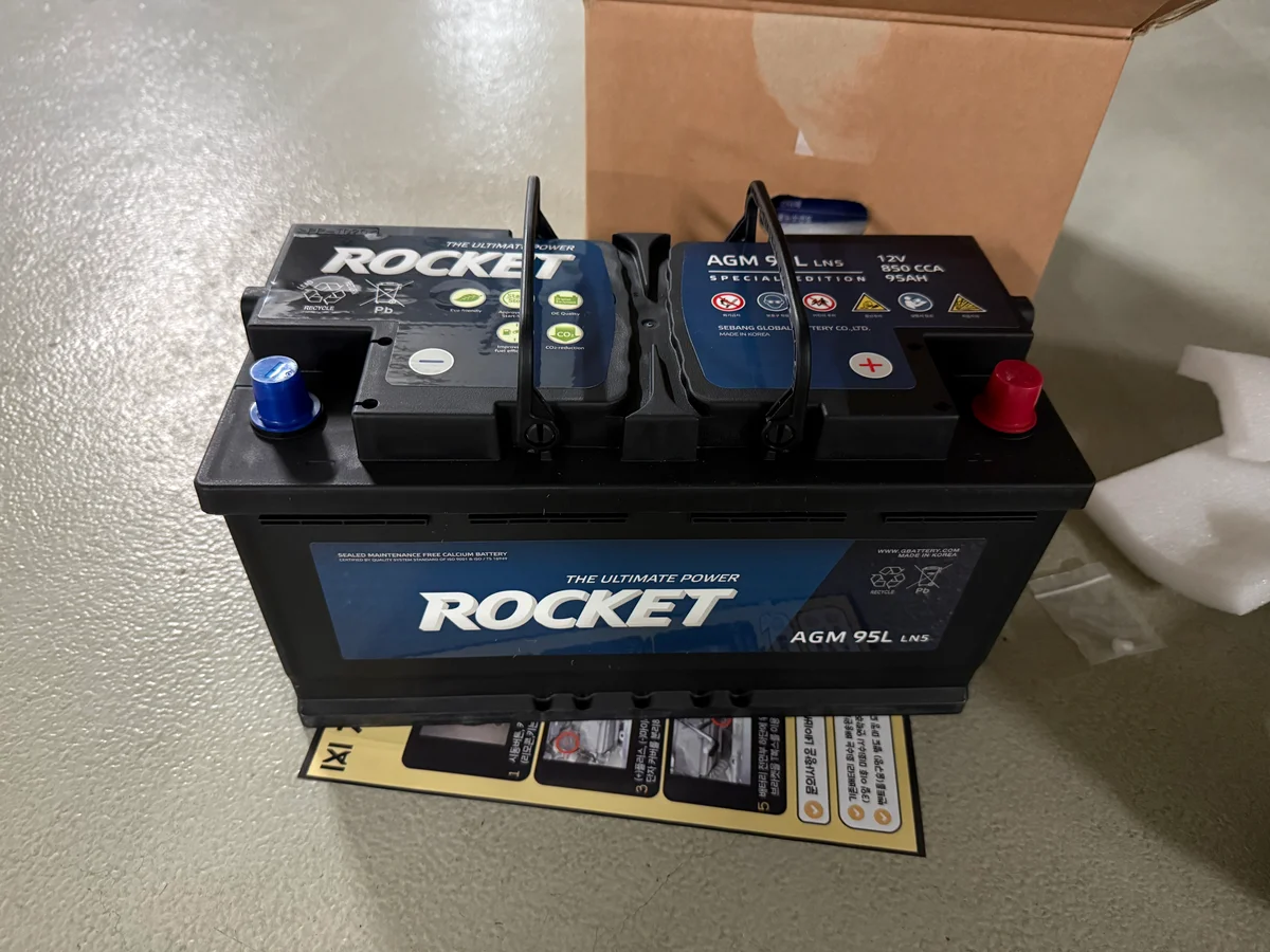
실은 그냥 AGM 배터리로 교체할 당위성을 확보하기 위해서 근거 자료를 확보한 것뿐입니다. 생각보다 무겁고 비싼 배터리를 구매하는데 스스로 설득하기 위한 시뮬레이션이었습니다. 주문후 도착한 배터리를 교체하기 위해서 공구를 챙겨서 주차장으로 내려왔습니다.
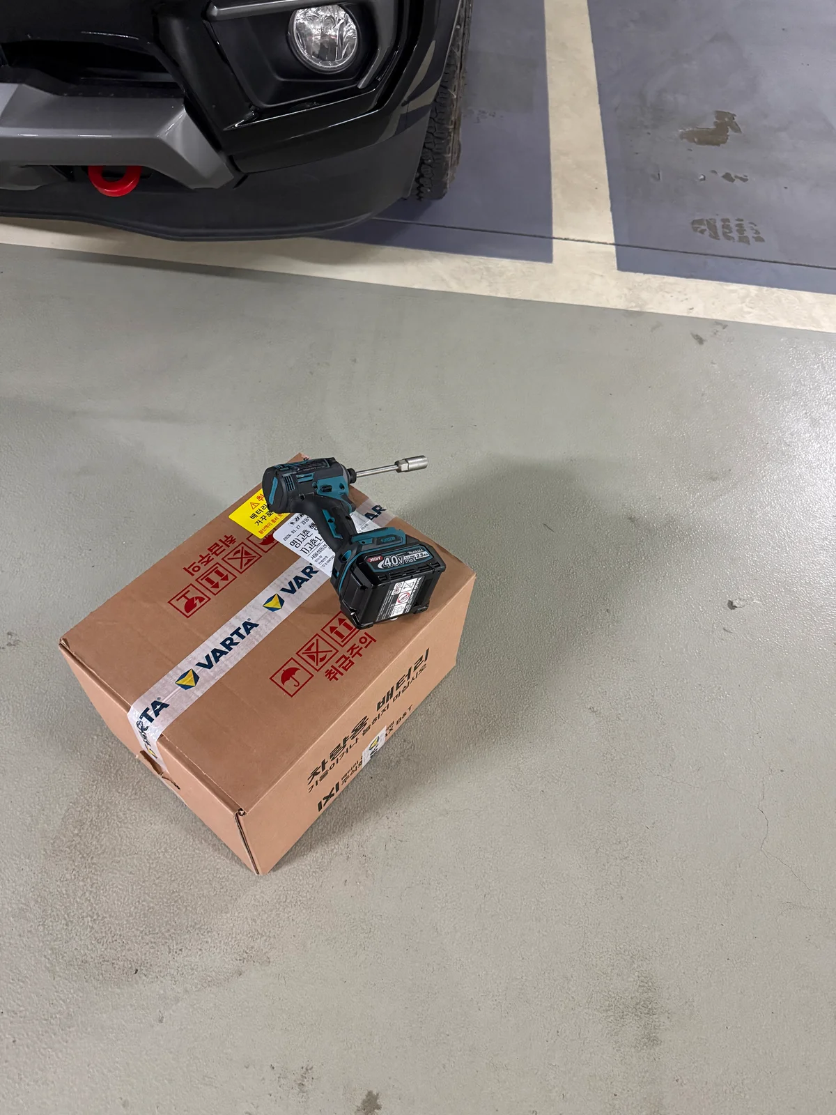
쉐비 콜로라도 배터리 고정 너트를 풀기 위해서는 13mm 복스(소켓)이 필요합니다. 그 외에는 장갑과 일자 드라이버 정도가 있으면 좋을듯 합니다.
교체 작업 순서
배터리 교체의 기본 원칙은 다음과 같습니다:
- 제거할 때: 마이너스(-) 먼저, 그 다음 플러스(+)
- 장착할 때: 플러스(+) 먼저, 그 다음 마이너스(-)
차량용 배터리의 전압이 12V이기에, 간과할 수 있지만 전류가 매우 높기 때문에 위 순서가 매우 중요합니다. 혹시라도 반대로 하신다면 불꽃이 보이거나, 단자가 열로 인하여 붙는 현상이 발생할 수 있고, 깜짝 놀랄 수 있습니다.
1. 기존 배터리 제거
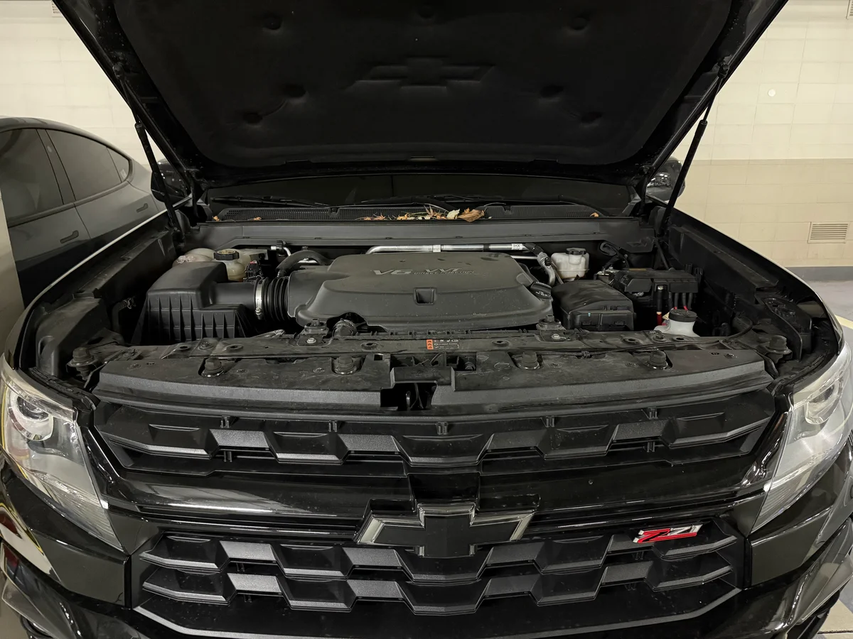
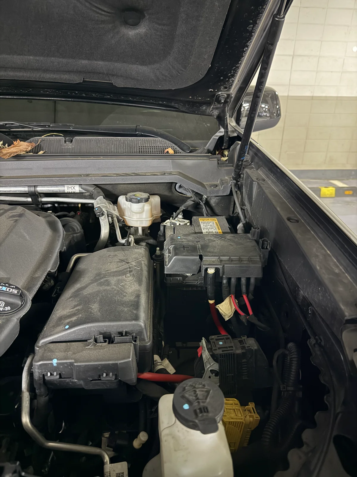
먼저 본넷을 열고 배터리 위치를 확인합니다.

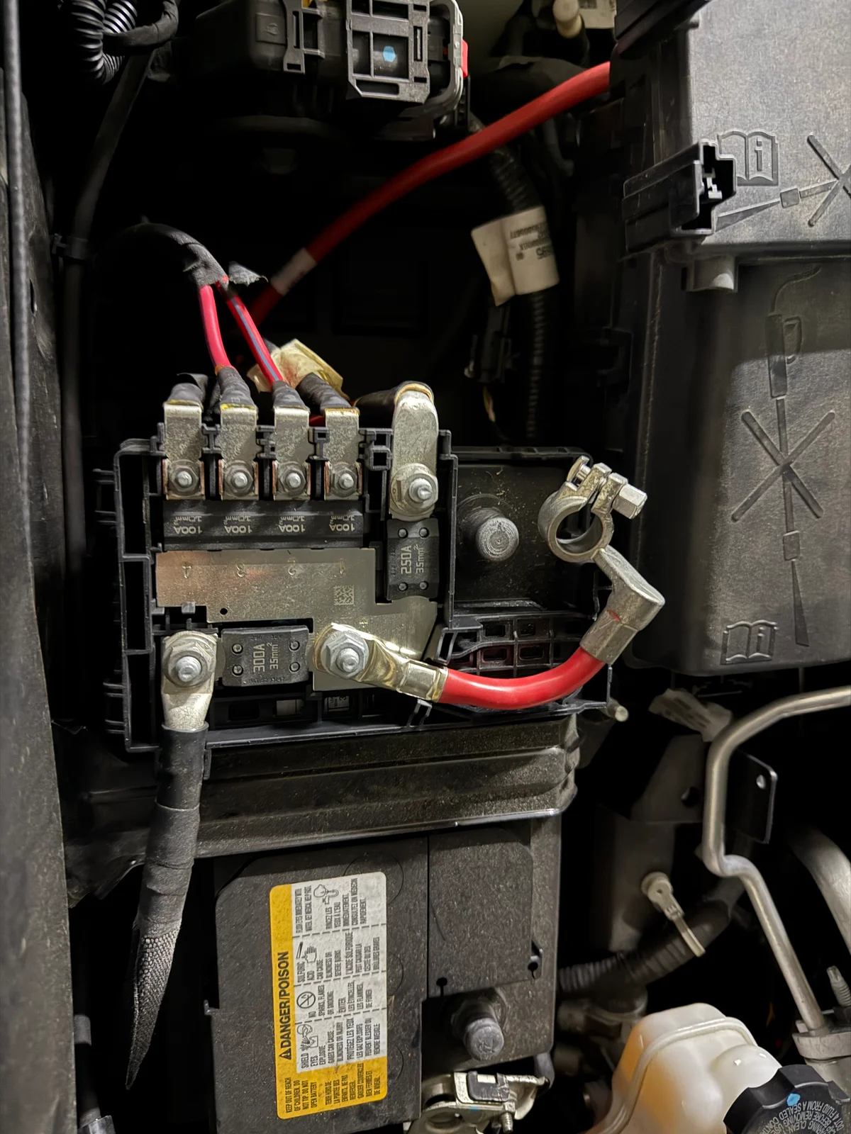
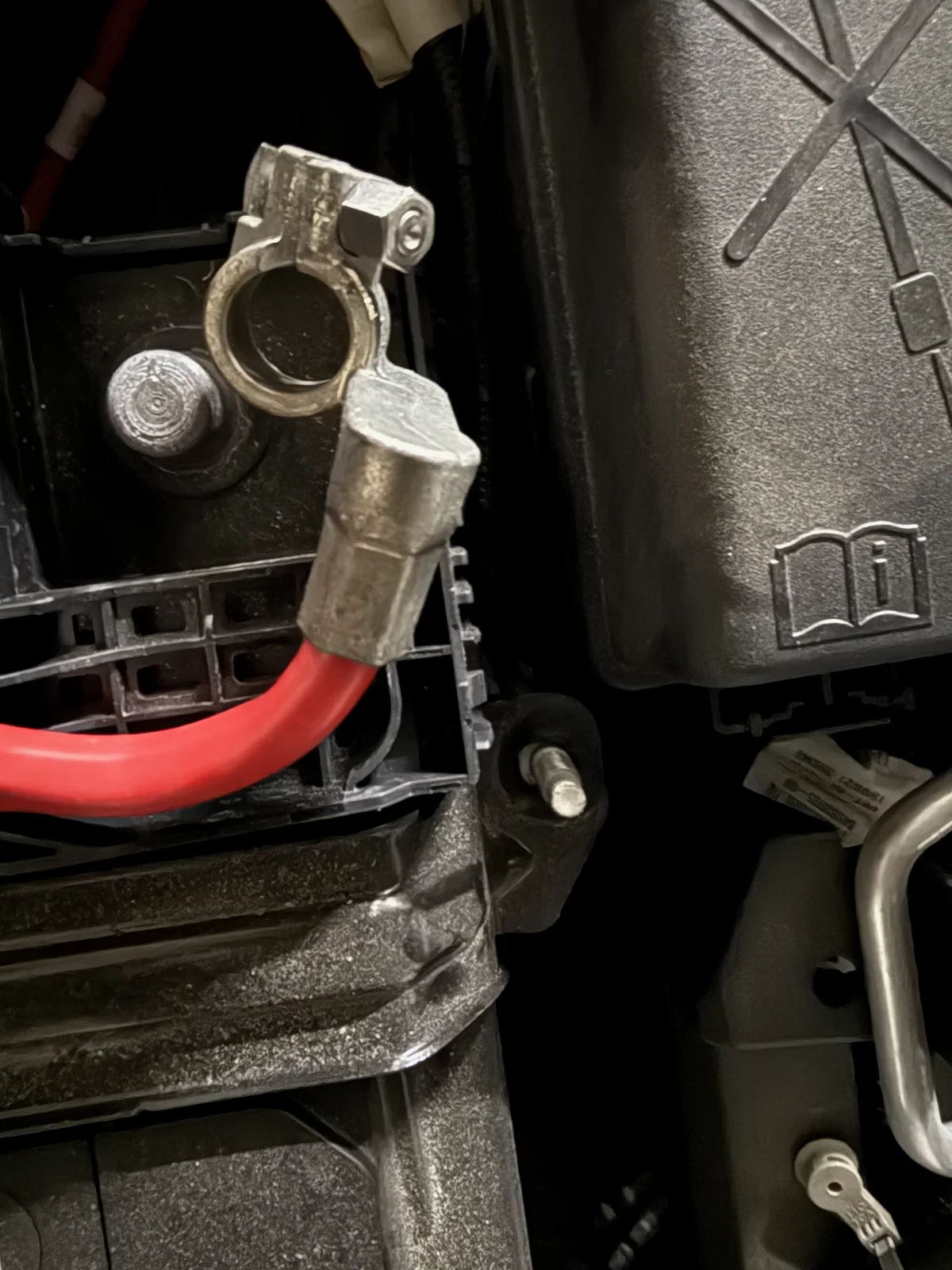
이제 배터리 마이너스 단자와 플러스 단자를 풀러줍니다.
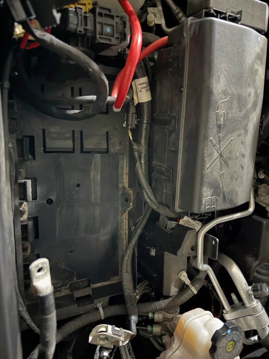
이제 배터리를 차체에 고정하고 있는 브라켓을 13mm 복스를 이용해 풀어줍니다. 보통 배터리 하단 깊숙한 곳에 있는데, 콜로라도는 그냥 위에 있습니다. T 복스라고 해서 엄청 기다란 도구가 필요할 줄 알았는데, 그냥 일반 스패너로도 풀리는 위치에 있었습니다.
배터리 브라켓을 풀고 나면, 엄청나게 무거운 배터리를 들어 올려 탈거할 수 있습니다.
2. 새 배터리 장착
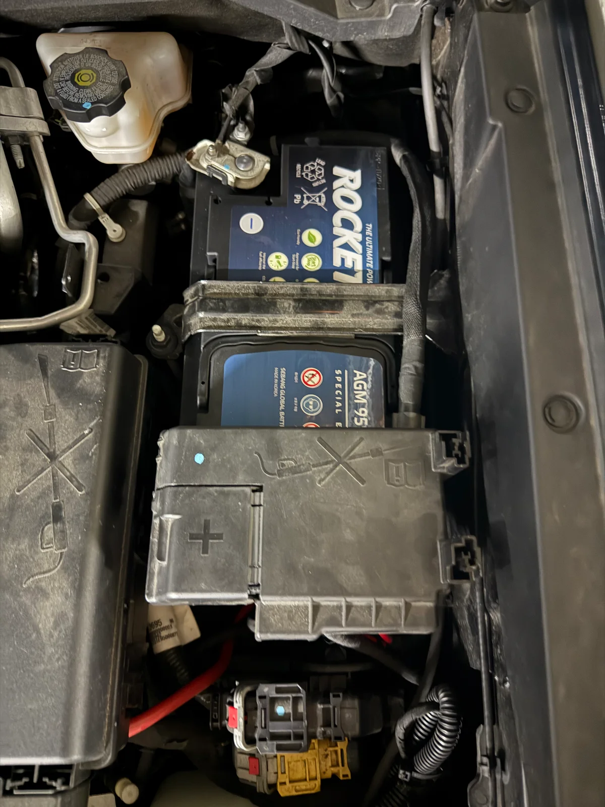
새 배터리의 포장을 뜯어 장착을 준비했습니다. 기존 납산 배터리보다 용량이 더 크니, 무게도 더 무겁고 크기도 더 큽니다. 다행인건 배터리 자체에 손잡이가 있어서 혼자서 간신히 들수 있었습니다.
규격이 조금 달라졌지만 트레이에 여유가 있어서 잘 들어갈 수 있었습니다. 다만, 전선들이 얽혀있어서 조금 정리가 필요했습니다.
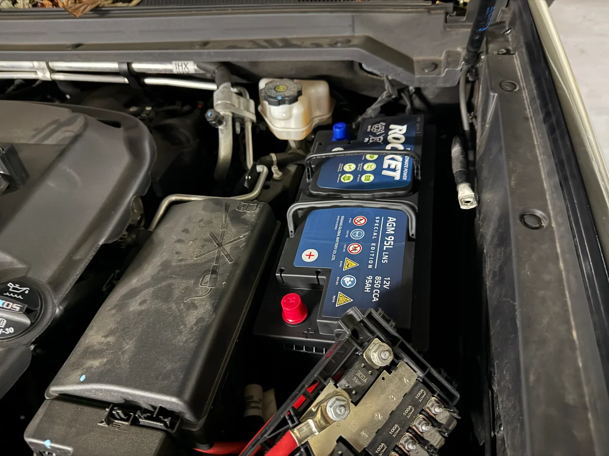
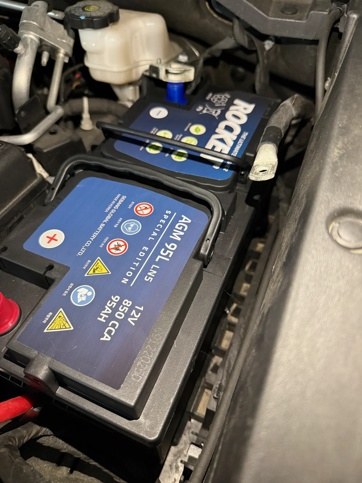
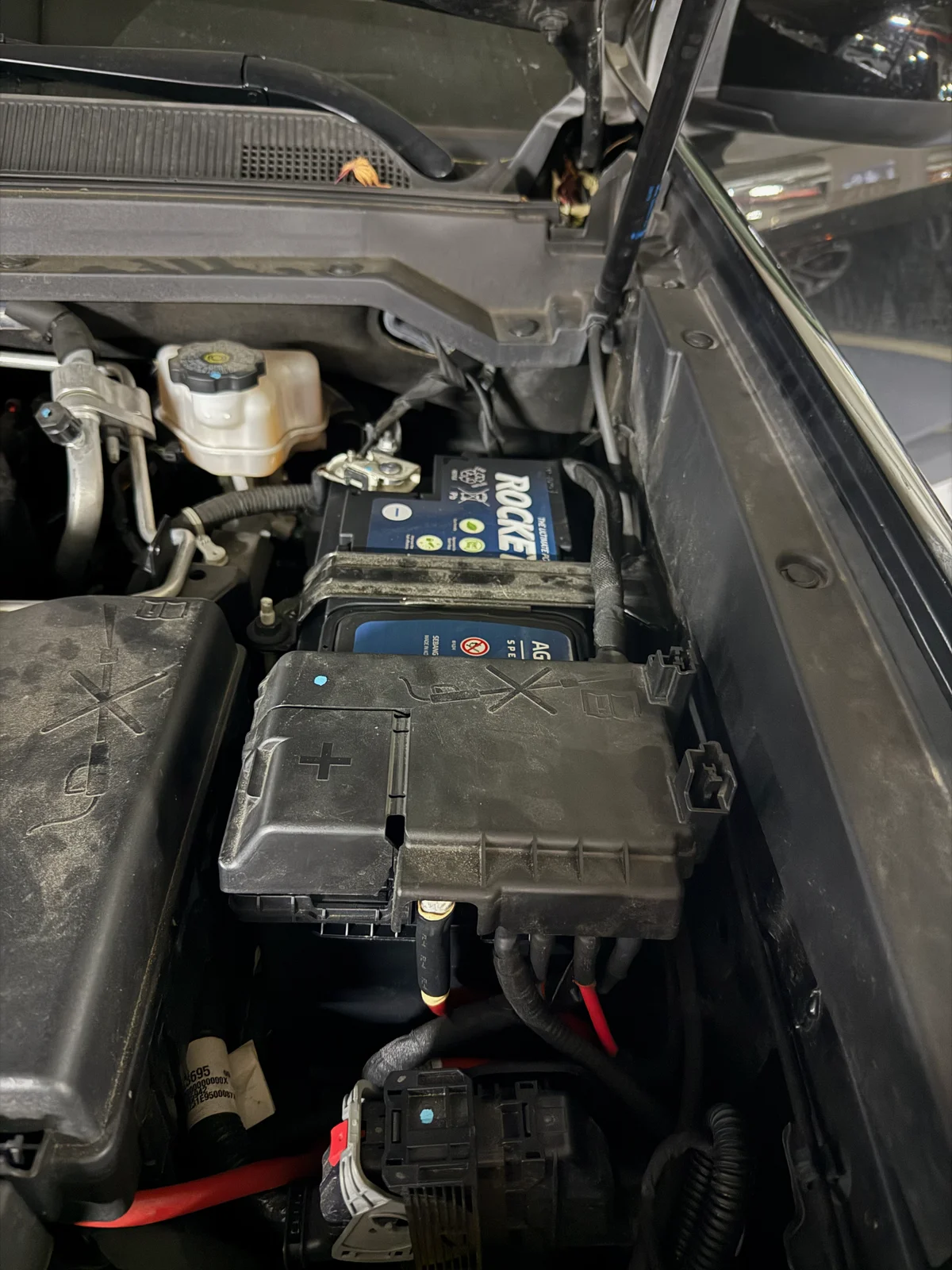
3. 단자 연결 및 브라켓 고정
단자가 단단히 고정되었는지 흔들어보고, 브라켓까지 고정하여 마무리합니다.
마무리
정말 다행이도 교체 후 시동이 걸렸습니다. 이제는 수행해본 시뮬레이션이 제대로 맞는지 검증해보는 일만 남았습니다.
Subscribe via RSS
Comments